COGITO Tutorials

These tutorials cover installing the COGITO code, running the main COGITO code, and analyzing bonding with the COGITO tight binding model. The workflow below provides the general outline. Click the section labels to quickly get to each section.

Installation

bash

pip install --upgrade pip
pip install cogito-dft

To install optional dependences (scikit-image, dash, dash-ag-grid) that are used in some COGITOpost functions:

bash

pip install "cogito-dft[plot]"

To avoid thread oversubscription and possible stalls (especially on HPC), set:

bash

export OMP_NUM_THREADS=1

Standard Workflow

VASP

tutorial.html#run-vasp

→

COGITO

tutorial.html#run-cogito

→

Check quality

tutorial.html#analyze-quality-of-cogito-run

→

Gain chemical insight

tutorial.html#generate-atom-and-bond-data

Run VASP

A couple things to keep in mind for the VASP calculation:

• Must be a static run (NSW=0)

• Use an irreducible grid (ISYM=1,2,3)

• Save the wavefunctions (LWAVE=True)

• Use more bands (NBANDS=(8-16)*natoms)

• No spin-orbit coupling (LSORBIT=False, but magnetism is supported (ISPIN=2)

Run COGITO

Execute the main COGITO code that adapts the atomic orbital basis and calculates the corresponding Hamiltonian matrix.

COGITO reads the POSCAR, POTCAR, OUTCAR, vasprun.xml, and WAVECAR files from the VASP calculation. For more on inputs and outputs of the main COGITO module, see COGITO files.

bash (CLI)

COGITO --dir "Si/"

python

from COGITO_dft.COGITO import run_cogito

direct = "Si/"
run_cogito(directory=direct)

Analyze quality of COGITO run

Checkes if quality output files are within expected range. If not, suggests tag changes that could improve quality. Run after COGITOpost for feedback on band interpolation quality. For more details, see COGITOanalyze files.

bash (CLI)

COGITOanalyze --dir "Si/"

python

from COGITO_dft.COGITOanalyze import analyze_all

direct = "Si/"
analyze_all(dir=direct)

Study COGITO model

To run the general model analysis:

bash (CLI)

COGITOpost --dir "Si/"

python

from COGITO_dft.COGITOpost import run_cogito_model

direct = "Si/"
run_cogito_model(directory=direct)

This general analysis can be broken into 4 parts: 1) Create class and plot decay of overlap/TB parameters, 2) Check band interpolation error compared to DFT, 3) Generate integrated atom and bond projected data, and 4) Generate the crystal bonds and/or combined bond and COHP projected density of states plots.

For a better understanding of the structure of the data, review Section VI of the COGITO manuscript.

These 4 parts can be customized with tags in command line interface or run in python individually, as reviewed below. For more a detailed analysis on density of states (uniform k-grid) or band structue, see below, explore COGITOpost files, or reference the API/source code.

1) Create COGITO TB class object and check decay

Now we can work with our COGITO tight binding model. The first step is to verify the quality of the COGITO TB model.

python

This code will need to be run before any use of the bandstructure or uniform classes.

from COGITO_dft.COGITOpost import COGITO_TB_Model as CoTB

direct = "Si/"
# create TB class from a directory that has run COGITO
my_CoTB = CoTB(direct)
my_CoTB.normalize_params() # for precise normalization
# restrict the TB parameters to improve speed
my_CoTB.restrict_params(maximum_dist=15, minimum_value=0.00001)

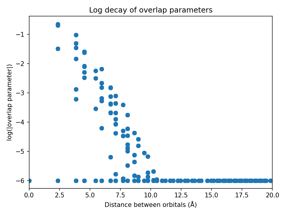
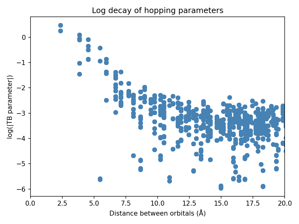
# optionally, plot the overlap and hopping parameters to check decay
my_CoTB.plot_overlaps(my_CoTB) # generates overlaps_decay.png
my_CoTB.plot_hoppings(my_CoTB) # generates tbparams_decay.png

Note: The overlap and hopping plots should show a rough linear decay

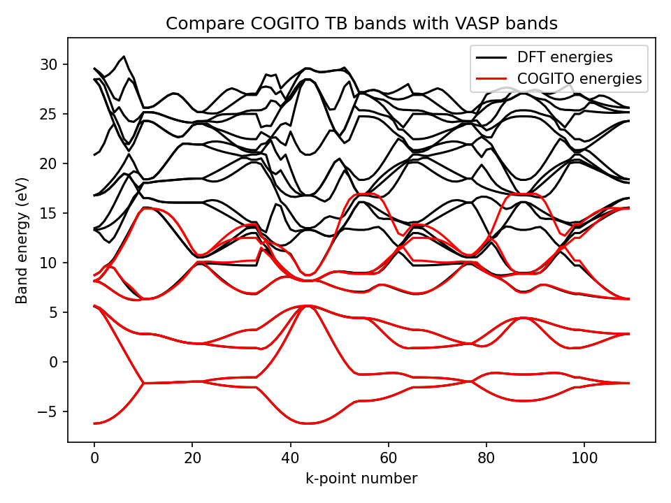
2) Compare COGITO band energies to DFT

To verify the band interpolation of COGITO, the function ‘compare_to_DFT’ is used to determine the error between the interpolating COITO band energies and DFT band energies. The DFT energies are read from an EIGENVAL file from a VASP (band structure) calculation.

bash (CLI)

COGITOpost --dir "Si/" --eigfile 'EIGENVAL' --no_save_crystal_bonds --no_save_bondswCOHP --no_save_ico

python

# the EIGENVAL file you want to compare to
eig_file = my_CoTB.directory + "EIGENVAL"
# generates compareDFT.png and DFT_band_error.txt
[band_dist, max_error, band_error] = CoTB.compare_to_DFT( my_CoTB, eig_file)

Metrics for the fit quality will be printed and written to the DFT_band_error.txt as below.

File generated by COGITO TB
average error in Valence Bands: 0.006377 eV
band distance in Valence Bands: 0.011352 eV
max error in valence band: 0.053859 eV
average error in Bottom 3 eV of CB: 0.017887 eV
average error in Conduc Bands: 0.357561 eV

3) Generate atom and bond data

By paritioning integrated values (like charge and band energy) into atom and bond contributions, we generate three json data files. These json files contain almost everything you may want to analyze! (Band structure or DOS analysis requires more effort.)

In the future, I will develop a more thorough tutorial of these files with examples of how to use them, but for now reference COGITOpost files, examine the files yourself, and email me (Emily) with any questions.

bash (CLI)

COGITOpost --dir "Si/" --densify 1.0  --no_save_quality_info --no_save_crystal_bonds --no_save_bondswCOHP --no_save_ico

python

# first, make an object of the uniform class
from COGITO_dft.COGITOpost import COGITO_UNIFORM as CoUN
import numpy as np

densify = 1.0 # increase for better DOS plots
new_grid = np.array(np.around(np.array(my_CoTB.num_trans) * densify, decimals=0),dtype=int)
# new_grid = [10,10,10] # can also just set manually

my_CoUN = CoUN(my_CoTB, grid=new_grid) # create uniform class
min_cohp = 0.00001 # adjust to include more or less bonds in json data
my_CoUN.jsonify_bonddata(minimum_cohp=min_cohp)

4) Create interactive visualization of quantum bonds!

The accurate TB model from COGITO allows for calculation of COHP energies which accurately reflect the DFT energies. This can be used to confidently and precisely trace back the crystal covalent bonding.

bash (CLI)

COGITOpost --dir "Si/" --energy_cutoff 0.05 --bond_max 3 --auto_label 'mulliken' --no_save_quality_info --no_save_bondswCOHP --no_save_ico

python

# plot the crystal structure with real bonds!
# if a bond energy magnitude is > energy_cutoff it will be plotted
# if the bond length is > bond_max it will not be plotted if an atom is outside the primitive cell
my_CoUN.get_bonds_charge_figure(energy_cutoff=0.05, bond_max=3, auto_label="mulliken")

bash (CLI)

Note: It often good to set densify >1.0 for the COHP projected density of states plot.

COGITOpost --dir "PbO/" --densify 1.5 --energy_cutoff 0.05 --bond_max 3 --auto_label 'full' --no_save_quality_info --no_save_crystal_bonds --no_save_ico

python

# plot the crystal bonds plot with an interative projected COHP!
my_CoUN.get_crystal_plus_COHP(energy_cutoff=0.05, bond_max=3, auto_label="full")

Additional Analysis

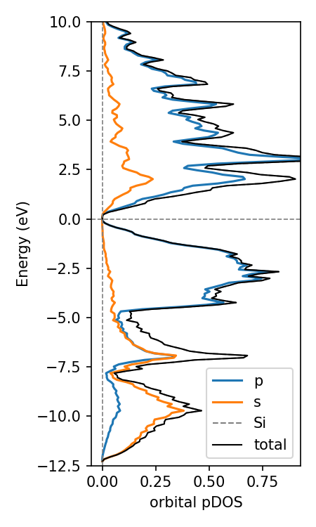
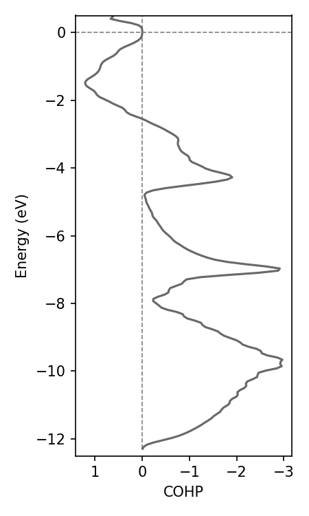
Orbital, COHP, or COOP projected DOS

Because COGITO forms a nearly complete basis for the charge density, we can accurately determine the percent of each atomic orbital in the band wavefunction. Mulliken population analysis is used here to resolve the inherit ambiguity in assigning two-center terms to one orbital.

The get_COHP function requires specifying two sets of orbitals. All bonds between an orbital in set 1 with an orbital in set 2 that also satisfy the nearest neighbor (NN) type are included in end COHP. The same function exists for COOP.

python

# make the unifom class object
from COGITO_dft.COGITOpost import COGITO_UNIFORM as CoUN
import numpy as np
densify = 1.0 # increase for better DOS plots
new_grid = np.array(np.around(np.array(my_CoTB.num_trans) * densify, decimals=0),dtype=int)
my_CoUN = CoUN(my_CoTB, grid=new_grid) # create uniform class

# Get orbital/element projected DOS for an element
my_CoUN.get_projectedDOS("Si",ylim=(-10,5),sigma=0.09) # sigma is gaussian smearing, adjust with initial k-grid

# specify the two sets as a list of two dictionaries
# in the dictionary, the keys are elements, and the values are the orbitals included for that atom
# each dictionary can have multiple atoms as keys, example for PbO
# orbs_dict = [{"Pb":["s","p","d"],"O":["s","p","d"]},{"Pb":["s","p","d"],"O":["s","p","d"]}]
# alternatively, list the orbital indices that you want to include (get from all_bonds.json)
# orbs_dict = [[0,1,2,3],[4,5,6,7]] # include bonds between the first silicon atom and second silicon atom

orbs_dict = [{"Si":["s","p","d"]},{"Si":["s","p","d"]}] # for silicon
my_CoUN.get_COHP(orbs_dict, NN='All')

Generate and project on band structure

This class generates the band structure for high symmetry path determined with pymatgen and seekpath. Importantly, this class requires an instance of the tight binding class in initialization.

python

# ensure TB class object is made
from COGITO_dft.COGITOpost import COGITO_TB_Model as CoTB
direct = "Si/"
my_CoTB = CoTB(direct) # create class from directory
my_CoTB.normalize_params() # for precise normalization
my_CoTB.restrict_params(maximum_dist=15, minimum_value=0.00001)

# now create band structure
from COGITO_dft.COGITOpost import COGITO_BAND as CoBS
my_CoBS = CoBS(my_CoTB, num_kpts = 10) # num_kpts is actually num per line, so set low
# plot band structure
my_CoBS.plotBS() # or plotlyBS()

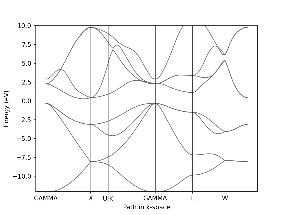
Use COGITO for orbital projected band structure
Because COGITO forms a nearly complete basis for the charge density, we can accurately determine the percent of each atomic orbital in the band wavefunction. Mulliken population analysis is used here to resolve the inherit ambiguity in assigning two-center terms to one orbital.

python

# plot the projected band structure of Si s orbitals
my_CoBS.get_projectedBS({"Si":["s"]})

Use COGITO for COHP/COOP projected band structure
The accurate TB model from COGITO allows for calculation of COHP energies which almost perfectly reflect the true DFT values. This can be used to confidently and precisely trace back the crystal chemical origins of electronic structure!

Any COHP requires specifying two sets of orbitals. The bonds between any orbital in set 1 with any orbital in set 2 is included in end COHP.

python

# specify the two sets as a list of two dictionaries
# in the dictionary, the keys are elements, and the values are the orbitals included for that atom
# each dictionary can have multiple atoms as keys, example for PbO
# orbs_dict = [{"Pb":["s","p","d"],"O":["s","p","d"]},{"Pb":["s","p","d"],"O":["s","p","d"]}]
# alternatively, list the orbital indices that you want to include (get from all_bonds.json)
# orbs_dict = [[0,1,2,3],[4,5,6,7]] # include bonds between the first silicon atom and second silicon atom

orbs_dict = [{"Si":["s","p","d"]},{"Si":["s","p","d"]}] # for silicon
my_CoBS.get_COHP(orbs_dict, NN='All')

# bonus points for running the interactive dash app
# this populates the autogenerates options for orbs_dict for the user to choose from
my_CoBS.make_COHP_dashapp()